In the previous Data Structure lesson we reviewed vectors, matrices, and arrays. And now in this lesson we will review:
- Data frames
- Tibbles
Data frames
- A data frame is a common way of storing data in R.
- In data frames, the columns are the different variables of the data set and the rows are unique observations.
- This may sound similar to matrices, but matrices can only have one type of data.
- Data frames can have variables of different types. For example, one variable may be a character and one may be numeric.
- R has several built-in data sets formatted into data frames (e.g.,
mtcars,iris,toothgrowth, and more).
mtcars example
Let’s take a look at mtcars:
mtcars mpg cyl disp hp drat wt qsec vs am gear
Mazda RX4 21.0 6 160.0 110 3.90 2.620 16.46 0 1 4
Mazda RX4 Wag 21.0 6 160.0 110 3.90 2.875 17.02 0 1 4
Datsun 710 22.8 4 108.0 93 3.85 2.320 18.61 1 1 4
Hornet 4 Drive 21.4 6 258.0 110 3.08 3.215 19.44 1 0 3
Hornet Sportabout 18.7 8 360.0 175 3.15 3.440 17.02 0 0 3
Valiant 18.1 6 225.0 105 2.76 3.460 20.22 1 0 3
Duster 360 14.3 8 360.0 245 3.21 3.570 15.84 0 0 3
Merc 240D 24.4 4 146.7 62 3.69 3.190 20.00 1 0 4
Merc 230 22.8 4 140.8 95 3.92 3.150 22.90 1 0 4
Merc 280 19.2 6 167.6 123 3.92 3.440 18.30 1 0 4
Merc 280C 17.8 6 167.6 123 3.92 3.440 18.90 1 0 4
Merc 450SE 16.4 8 275.8 180 3.07 4.070 17.40 0 0 3
Merc 450SL 17.3 8 275.8 180 3.07 3.730 17.60 0 0 3
Merc 450SLC 15.2 8 275.8 180 3.07 3.780 18.00 0 0 3
Cadillac Fleetwood 10.4 8 472.0 205 2.93 5.250 17.98 0 0 3
Lincoln Continental 10.4 8 460.0 215 3.00 5.424 17.82 0 0 3
Chrysler Imperial 14.7 8 440.0 230 3.23 5.345 17.42 0 0 3
Fiat 128 32.4 4 78.7 66 4.08 2.200 19.47 1 1 4
Honda Civic 30.4 4 75.7 52 4.93 1.615 18.52 1 1 4
Toyota Corolla 33.9 4 71.1 65 4.22 1.835 19.90 1 1 4
Toyota Corona 21.5 4 120.1 97 3.70 2.465 20.01 1 0 3
Dodge Challenger 15.5 8 318.0 150 2.76 3.520 16.87 0 0 3
AMC Javelin 15.2 8 304.0 150 3.15 3.435 17.30 0 0 3
Camaro Z28 13.3 8 350.0 245 3.73 3.840 15.41 0 0 3
Pontiac Firebird 19.2 8 400.0 175 3.08 3.845 17.05 0 0 3
Fiat X1-9 27.3 4 79.0 66 4.08 1.935 18.90 1 1 4
Porsche 914-2 26.0 4 120.3 91 4.43 2.140 16.70 0 1 5
Lotus Europa 30.4 4 95.1 113 3.77 1.513 16.90 1 1 5
Ford Pantera L 15.8 8 351.0 264 4.22 3.170 14.50 0 1 5
Ferrari Dino 19.7 6 145.0 175 3.62 2.770 15.50 0 1 5
Maserati Bora 15.0 8 301.0 335 3.54 3.570 14.60 0 1 5
Volvo 142E 21.4 4 121.0 109 4.11 2.780 18.60 1 1 4
carb
Mazda RX4 4
Mazda RX4 Wag 4
Datsun 710 1
Hornet 4 Drive 1
Hornet Sportabout 2
Valiant 1
Duster 360 4
Merc 240D 2
Merc 230 2
Merc 280 4
Merc 280C 4
Merc 450SE 3
Merc 450SL 3
Merc 450SLC 3
Cadillac Fleetwood 4
Lincoln Continental 4
Chrysler Imperial 4
Fiat 128 1
Honda Civic 2
Toyota Corolla 1
Toyota Corona 1
Dodge Challenger 2
AMC Javelin 2
Camaro Z28 4
Pontiac Firebird 2
Fiat X1-9 1
Porsche 914-2 2
Lotus Europa 2
Ford Pantera L 4
Ferrari Dino 6
Maserati Bora 8
Volvo 142E 2- R returns the entire data frame, so if you’re like me and like to view your output in the console of RStudio, you’ll probably need to scroll up in order to see first row along with the variables.
- We can see there are 11 variables, but it’s hard to know exactly how many rows (or observations) there are.
- We can type
?mtcarsinto the console to get more information. - Here, we can see there are 32 observations and we can see what each variable is.
Helpful Functions to Explore Data Frame
We can also use existing functions to help us understand our data better:
head()returns the top 6 rows. This doesn’t actually give us any new information about our data set, but it’s a really useful function to know about because it’s helpful to be able to get a view of the first several rows along with the variable names.
head(mtcars) mpg cyl disp hp drat wt qsec vs am gear carb
Mazda RX4 21.0 6 160 110 3.90 2.620 16.46 0 1 4 4
Mazda RX4 Wag 21.0 6 160 110 3.90 2.875 17.02 0 1 4 4
Datsun 710 22.8 4 108 93 3.85 2.320 18.61 1 1 4 1
Hornet 4 Drive 21.4 6 258 110 3.08 3.215 19.44 1 0 3 1
Hornet Sportabout 18.7 8 360 175 3.15 3.440 17.02 0 0 3 2
Valiant 18.1 6 225 105 2.76 3.460 20.22 1 0 3 1View()allows you to view the data frame in a new window, making it easier to explore the full data set.
View(mtcars)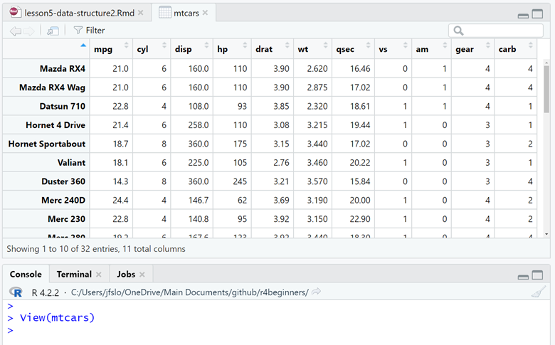
nrow()returns the total number of rows in your data frame.
nrow(mtcars)[1] 32ncol()returns the total number of columns in your data frame.
ncol(mtcars)[1] 11str()returns the “structure” of our data frame in a compact way.
- We can see the number of observations and number of variables.
- We can also see a bit more information about each variable. For example, we can see that all of the variables in
mtcarsare numeric. It even lists the first several observations for each variable. glimpse()is a similar function tostr(). I encourage you to try it out!
str(mtcars)'data.frame': 32 obs. of 11 variables:
$ mpg : num 21 21 22.8 21.4 18.7 18.1 14.3 24.4 22.8 19.2 ...
$ cyl : num 6 6 4 6 8 6 8 4 4 6 ...
$ disp: num 160 160 108 258 360 ...
$ hp : num 110 110 93 110 175 105 245 62 95 123 ...
$ drat: num 3.9 3.9 3.85 3.08 3.15 2.76 3.21 3.69 3.92 3.92 ...
$ wt : num 2.62 2.88 2.32 3.21 3.44 ...
$ qsec: num 16.5 17 18.6 19.4 17 ...
$ vs : num 0 0 1 1 0 1 0 1 1 1 ...
$ am : num 1 1 1 0 0 0 0 0 0 0 ...
$ gear: num 4 4 4 3 3 3 3 4 4 4 ...
$ carb: num 4 4 1 1 2 1 4 2 2 4 ...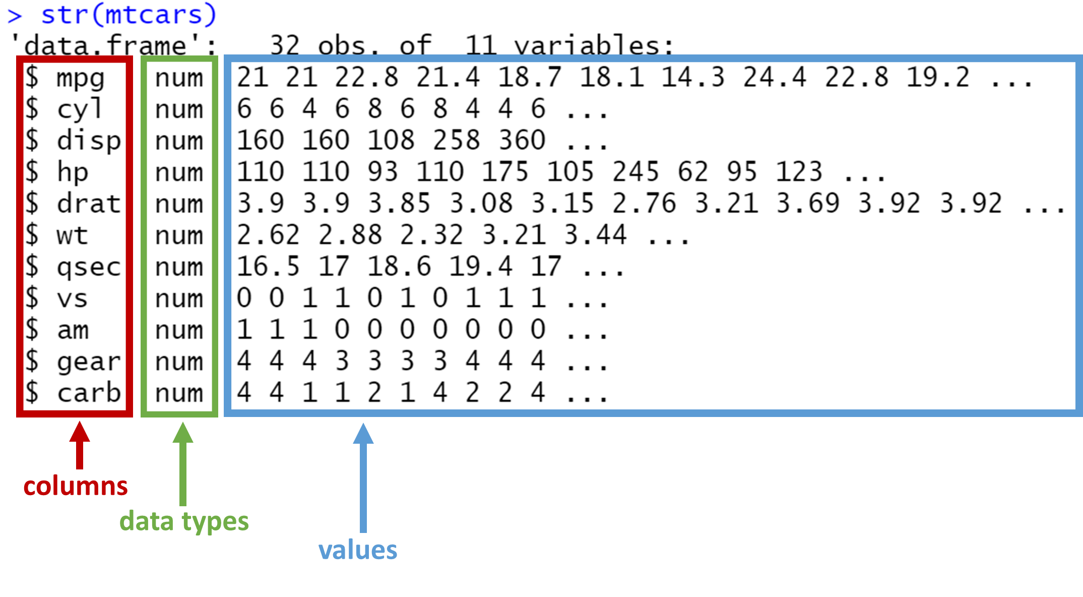
summary()provides a summary of the different variables. Because all the variables are numeric, we can see the summary function returns the following information: minimum value, 1st quartile (25th percentile), median, mean, 3rd quartile (75th percentile), and maximum value.
summary(mtcars) mpg cyl disp hp
Min. :10.40 Min. :4.000 Min. : 71.1 Min. : 52.0
1st Qu.:15.43 1st Qu.:4.000 1st Qu.:120.8 1st Qu.: 96.5
Median :19.20 Median :6.000 Median :196.3 Median :123.0
Mean :20.09 Mean :6.188 Mean :230.7 Mean :146.7
3rd Qu.:22.80 3rd Qu.:8.000 3rd Qu.:326.0 3rd Qu.:180.0
Max. :33.90 Max. :8.000 Max. :472.0 Max. :335.0
drat wt qsec vs
Min. :2.760 Min. :1.513 Min. :14.50 Min. :0.0000
1st Qu.:3.080 1st Qu.:2.581 1st Qu.:16.89 1st Qu.:0.0000
Median :3.695 Median :3.325 Median :17.71 Median :0.0000
Mean :3.597 Mean :3.217 Mean :17.85 Mean :0.4375
3rd Qu.:3.920 3rd Qu.:3.610 3rd Qu.:18.90 3rd Qu.:1.0000
Max. :4.930 Max. :5.424 Max. :22.90 Max. :1.0000
am gear carb
Min. :0.0000 Min. :3.000 Min. :1.000
1st Qu.:0.0000 1st Qu.:3.000 1st Qu.:2.000
Median :0.0000 Median :4.000 Median :2.000
Mean :0.4062 Mean :3.688 Mean :2.812
3rd Qu.:1.0000 3rd Qu.:4.000 3rd Qu.:4.000
Max. :1.0000 Max. :5.000 Max. :8.000 - What if we only wanted to get a summary of the first variable, mpg? No problem, we can modify the code like this:
summary(mtcars$mpg) Min. 1st Qu. Median Mean 3rd Qu. Max.
10.40 15.43 19.20 20.09 22.80 33.90 Tibbles
A tibble is a type of data frame with some special features that we will explore. If you use tidyverse, chances our you’ll see a lot of tibbles!
There are some differences between tibbles and data frames, but those are not important when learning the basics. We’ll go through the basic differences, but here’s a useful link if you’re interested in learning more about tibbles: tibble.tidyverse.org.
Penguins example
To understand the unique features of a tibble, we’ll explore the penguins data set that is included in the palmerpenguins package.
In the last lesson, we learned about packages. We know the first things we need to do is load the package and then we will have access to the penguins data set.
library(palmerpenguins)
penguins
# A tibble: 344 × 8
species island bill_length_mm bill_depth_mm flipper_length_mm
<fct> <fct> <dbl> <dbl> <int>
1 Adelie Torgersen 39.1 18.7 181
2 Adelie Torgersen 39.5 17.4 186
3 Adelie Torgersen 40.3 18 195
4 Adelie Torgersen NA NA NA
5 Adelie Torgersen 36.7 19.3 193
6 Adelie Torgersen 39.3 20.6 190
7 Adelie Torgersen 38.9 17.8 181
8 Adelie Torgersen 39.2 19.6 195
9 Adelie Torgersen 34.1 18.1 193
10 Adelie Torgersen 42 20.2 190
# … with 334 more rows, and 3 more variables: body_mass_g <int>,
# sex <fct>, year <int>- The first line of output says: “A tibble: 344 x 8”. Straight away, we get confirmation that this data frame is a tibble. And there are 344 rows and 8 columns.
- Because tibbles are a type of data frame, similar to what we saw with the
mtcarsdata frame, each column is a variable and each row is a unique observation. - Just to confirm, we can run the following 2 lines of code to see that penguins is both a data frame and a tibble:
Note: is_tibble() is a function in the tibble package, which is part of tidyverse, so we need to load in the tidyverse library first.
So what is special about tibbles?
- Tibbles are simple data frames with some features that make working with the data really nice.
- As already pointed out, the tibble shows us exactly how big our data set is (344 rows and 8 columns).
- It automatically only prints out the first 10 rows, so it’s much easier to see the variables in our data set.
- Under each variable name, we see what type of variable it is (e.g., fct, dbl, int, etc.)
- As a small aside, tidyverse uses “dbl” (“double”) instead of “numeric”, but they are identical.
- R only returns the number of columns that fit on your screen. For example, if you view your output in the console, it’s likely that not all of the variables will neatly fit on your screen. Under the 10 rows of data, you may see something like: “and 1 more variable: year
”. This is great because you get important information on all of the variables even if there are too many to fit on your screen.
Converting a data frame to a tibble
- Recall, that by default mtcars is a data frame and not a tibble,
mtcars mpg cyl disp hp drat wt qsec vs am gear
Mazda RX4 21.0 6 160.0 110 3.90 2.620 16.46 0 1 4
Mazda RX4 Wag 21.0 6 160.0 110 3.90 2.875 17.02 0 1 4
Datsun 710 22.8 4 108.0 93 3.85 2.320 18.61 1 1 4
Hornet 4 Drive 21.4 6 258.0 110 3.08 3.215 19.44 1 0 3
Hornet Sportabout 18.7 8 360.0 175 3.15 3.440 17.02 0 0 3
Valiant 18.1 6 225.0 105 2.76 3.460 20.22 1 0 3
Duster 360 14.3 8 360.0 245 3.21 3.570 15.84 0 0 3
Merc 240D 24.4 4 146.7 62 3.69 3.190 20.00 1 0 4
Merc 230 22.8 4 140.8 95 3.92 3.150 22.90 1 0 4
Merc 280 19.2 6 167.6 123 3.92 3.440 18.30 1 0 4
Merc 280C 17.8 6 167.6 123 3.92 3.440 18.90 1 0 4
Merc 450SE 16.4 8 275.8 180 3.07 4.070 17.40 0 0 3
Merc 450SL 17.3 8 275.8 180 3.07 3.730 17.60 0 0 3
Merc 450SLC 15.2 8 275.8 180 3.07 3.780 18.00 0 0 3
Cadillac Fleetwood 10.4 8 472.0 205 2.93 5.250 17.98 0 0 3
Lincoln Continental 10.4 8 460.0 215 3.00 5.424 17.82 0 0 3
Chrysler Imperial 14.7 8 440.0 230 3.23 5.345 17.42 0 0 3
Fiat 128 32.4 4 78.7 66 4.08 2.200 19.47 1 1 4
Honda Civic 30.4 4 75.7 52 4.93 1.615 18.52 1 1 4
Toyota Corolla 33.9 4 71.1 65 4.22 1.835 19.90 1 1 4
Toyota Corona 21.5 4 120.1 97 3.70 2.465 20.01 1 0 3
Dodge Challenger 15.5 8 318.0 150 2.76 3.520 16.87 0 0 3
AMC Javelin 15.2 8 304.0 150 3.15 3.435 17.30 0 0 3
Camaro Z28 13.3 8 350.0 245 3.73 3.840 15.41 0 0 3
Pontiac Firebird 19.2 8 400.0 175 3.08 3.845 17.05 0 0 3
Fiat X1-9 27.3 4 79.0 66 4.08 1.935 18.90 1 1 4
Porsche 914-2 26.0 4 120.3 91 4.43 2.140 16.70 0 1 5
Lotus Europa 30.4 4 95.1 113 3.77 1.513 16.90 1 1 5
Ford Pantera L 15.8 8 351.0 264 4.22 3.170 14.50 0 1 5
Ferrari Dino 19.7 6 145.0 175 3.62 2.770 15.50 0 1 5
Maserati Bora 15.0 8 301.0 335 3.54 3.570 14.60 0 1 5
Volvo 142E 21.4 4 121.0 109 4.11 2.780 18.60 1 1 4
carb
Mazda RX4 4
Mazda RX4 Wag 4
Datsun 710 1
Hornet 4 Drive 1
Hornet Sportabout 2
Valiant 1
Duster 360 4
Merc 240D 2
Merc 230 2
Merc 280 4
Merc 280C 4
Merc 450SE 3
Merc 450SL 3
Merc 450SLC 3
Cadillac Fleetwood 4
Lincoln Continental 4
Chrysler Imperial 4
Fiat 128 1
Honda Civic 2
Toyota Corolla 1
Toyota Corona 1
Dodge Challenger 2
AMC Javelin 2
Camaro Z28 4
Pontiac Firebird 2
Fiat X1-9 1
Porsche 914-2 2
Lotus Europa 2
Ford Pantera L 4
Ferrari Dino 6
Maserati Bora 8
Volvo 142E 2- However, we can easily use the
as_tibble()function to convert it to a tibble.
as_tibble(mtcars)# A tibble: 32 × 11
mpg cyl disp hp drat wt qsec vs am gear carb
<dbl> <dbl> <dbl> <dbl> <dbl> <dbl> <dbl> <dbl> <dbl> <dbl> <dbl>
1 21 6 160 110 3.9 2.62 16.5 0 1 4 4
2 21 6 160 110 3.9 2.88 17.0 0 1 4 4
3 22.8 4 108 93 3.85 2.32 18.6 1 1 4 1
4 21.4 6 258 110 3.08 3.22 19.4 1 0 3 1
5 18.7 8 360 175 3.15 3.44 17.0 0 0 3 2
6 18.1 6 225 105 2.76 3.46 20.2 1 0 3 1
7 14.3 8 360 245 3.21 3.57 15.8 0 0 3 4
8 24.4 4 147. 62 3.69 3.19 20 1 0 4 2
9 22.8 4 141. 95 3.92 3.15 22.9 1 0 4 2
10 19.2 6 168. 123 3.92 3.44 18.3 1 0 4 4
# … with 22 more rows- This example should highlight the advantages of working with tibbles.
- Personally, I try to work exclusively with tibbles because I find it so much easier and cleaner.
Create our own tibble
In the Data Structure: Part 1 lesson, we created three vectors: names, age, and blue_eyes. Now, let’s create a tibble consisting of these three vectors.
- We will use the
tibble()function. - Each line of our tibble represents a unique variable (or column). The text to the left of the equals sign is the variable name and the text to right is the data we want to be stored in our tibble. For example,
Nameis variable name for the first column and the data is ournamesvector (Josh, Jenny, Brandon). - We will save our tibble as
my_tibble().
names <- c("Josh", "Jenny", "Brandon")
ages <- c(31, 30, 27)
blue_eyes <- c(TRUE, FALSE, FALSE)

my_tibble <- tibble(
  Name = names,
  Age = ages,
  Blue_eye = blue_eyes
)

my_tibble
# A tibble: 3 × 3
Name Age Blue_eye
<chr> <dbl> <lgl>
1 Josh 31 TRUE
2 Jenny 30 FALSE
3 Brandon 27 FALSE - And just like that, we created our very own 3x3 tibble!
Summary
In this lesson we learned about data frames and tibbles. Data frames are one of the most common ways of storing data, where each column represents a variable and each row represents an observation. Tibbles are a type of data frame with special features that make it even easier to work with.
Exercises
- R has a built-in dataset called
airquality. Typeairqualityinto the R chunk below and run the code to see this data.
- Is this a standard data frame or is this a tibble? Use the
is.data.frame()andis_tibble()functions to confirm.
Hint: make sure you have the tidyverse library loaded before executing the `is_tibble() function.
- Now that we know
airqualityis not a tibble by default, use theas_tibble()function to convert it to a one.
Save this to a new variable called airquality_tibble.
Print airquality_tibble to see the results.
- Can you answer the following questions:
- How many columns does this dataset have?
- How many rows?
- What are the row names?
- What year are these data points from? Hint: use the help documentation by typing
?airqualityin the console.
Use the
View()to view the data in a new tab.Get the summary results of the wind variable.
- Find the average temperature of all the observations in this dataset.
THE END 🎉